< Probability and statistics definitions < Complementary cumulative distribution function
What is the complementary cumulative distribution function (CCDF)?
The complementary cumulative distribution function (CCDF) is defined in terms of the cumulative distribution function (CDF).
While the CDF is defined as
F(x) = P(X ≤ x),
the CCDF is defined as the complement of the CDF (i.e., 1 minus the CDF) [1]:
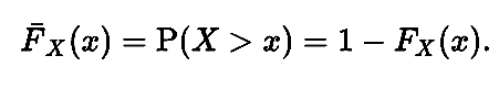
Therefore, the CCDF can be calculated from either the CDF or the probability density function (PDF).
CCDFs are sometimes called risk curves or survival functions. However, the survival function is the complementary cumulative distribution function of the lifetime — it gives the probability that a patient, device, or any object of interest will survive past a certain time — while any distribution (not just lifetimes) can have a CCDF. For example, the CCDF can be used to describe the distribution of income, the distribution of weights, or the distribution of meta distributions of random variables [2]. A meta distribution is a function that describes the distribution of other distributions, where each of the other distributions is a conditional distribution.
Complementary cumulative distribution example (discrete distribution)
Consider the following set of probabilities for mismatches in human genomes [3]:
| X | P(X) | CDF | CCDF |
| 0 | 0.6561 | 0.6561 | 0.3439 |
| 1 | 0.2916 | 0.9477 | 0.0523 |
| 2 | 0.0486 | 0.9963 | 0.0037 |
| 3 | 0.0036 | 0.9999 | 0.0001 |
| 4 | 0.0001 | 1.0000 | 0.0000 |
The probability mass function (PMF) in the second column gives us the probability that the number of mismatches is equal to X. For example, the probability that there are zero mismatches, P(x = 0), is 0.6561.
The CDF in the third column gives us the cumulative probabilities for the PMF. For example, F(2) = P(X ≤ 2) = P(X = 0) + P(X = 1) + P(X = 2) = 0.9963.
The complementary cumulative distribution function (CCDF) in the last column gives us the complement of the CDF. As the CDF is P(X ≤ x), its complement is P(X > x). For example, F>(2)= P(X >2) =1 ‐ P(X ≤ 2) = 0.0037.
References
[1] Myers, D. CS 547 Lecture 8: Continuous Random Variables.
[2] Haenggi, M. Meta Distributions—Part 1: Definition and Examples